Validation
A natural response when you get access to something someone else build is to wonder - does this work correctly?
This section will give you confidence in the implementation of underlying energy models.
Battery Validation
Price Dispatch Behaviour
Let's optimize a battery using a sequence of five prices.
We expect that the battery will charge when prices are low, and will discharge when prices are high.
In energypylinear, a positive site electricity balance is importing, and a negative site electricity balance is exporting.
import energypylinear as epl

asset = epl.Battery()
results = asset.optimize(electricity_prices=[10, -50, 200, -50, 200], verbose=False)
print(results.simulation[["electricity_prices", "site-electricity_balance_mwh"]])
   electricity_prices  site-electricity_balance_mwh
0                  10                      0.444444
1                 -50                      2.000000
2                 200                     -2.000000
3                 -50                      2.000000
4                 200                     -2.000000
As expected, the battery charges (with a site that is positive) when prices are low and discharges (with a negative site electricity balance) when prices are high.
Now let's change the prices and see how the dispatch changes:
import energypylinear as epl

asset = epl.Battery()
results = asset.optimize(electricity_prices=[200, -50, -50, 200, 200], verbose=False)
print(results.simulation[["electricity_prices", "site-electricity_balance_mwh"]])
As expected, the battery continues to charge during low electricity price intervals, and discharge when electricity prices are high.
Energy Balance
Let's return to our original set of prices and check the energy balance of the battery:
import pandas as pd
import energypylinear as epl

pd.set_option('display.max_columns', 15)
pd.set_option('display.width', 400)

asset = epl.Battery()
results = asset.optimize(electricity_prices=[10, -50, 200, -50, 200], verbose=False)

balance = epl.results.checks.check_electricity_balance(results.simulation, verbose=False)
print(balance)
      input  accumulation  output  raw_balance  balance    import  generation  export  load    charge  discharge      loss  spills  soc
0  0.444444     -0.444444     0.0         True     True  0.444444         0.0     0.0   0.0  0.444444        0.0  0.044444     0.0  0.0
1  2.000000     -2.000000     0.0         True     True  2.000000         0.0     0.0   0.0  2.000000        0.0  0.200000     0.0  0.0
2  0.000000      2.000000     2.0         True     True  0.000000         0.0     2.0   0.0  0.000000        2.0  0.000000     0.0  0.0
3  2.000000     -2.000000     0.0         True     True  2.000000         0.0     0.0   0.0  2.000000        0.0  0.200000     0.0  0.0
4  0.000000      2.000000     2.0         True     True  0.000000         0.0     2.0   0.0  0.000000        2.0  0.000000     0.0  0.0
In the first interval, we charge the battery with 0.444444 MWh - 0.4 MWh goes into increasing the battery state of charge from 0.0 MWh to 0.4 MWh, with the balance 0.044444 MWh going to battery losses.
Battery Efficiency
We can validate the performance of the battery efficiency by checking the losses across different battery efficiencies:
import numpy as np
import pandas as pd
import energypylinear as epl

out = []
np.random.seed(42)
prices = (np.random.uniform(-100, 100, 12) + 100).tolist()
for efficiency_pct in [1.0, 0.9, 0.8]:
    asset = epl.battery.Battery(
        power_mw=4,
        capacity_mwh=10,
        efficiency=efficiency_pct
    )
    results = asset.optimize(
        electricity_prices=prices,
        objective="price",
        verbose=False
    )
    out.append(
        {
            "eff_pct": efficiency_pct,
            "charge_mwh": results.simulation["battery-electric_charge_mwh"].sum(),
            "discharge_mwh": results.simulation["battery-electric_discharge_mwh"].sum(),
            "loss_mwh": results.simulation["battery-electric_loss_mwh"].sum(),
            "prices_$_mwh": results.simulation["electricity_prices"].mean(),
            "import_mwh": results.simulation["site-import_power_mwh"].sum(),
            "objective": (results.simulation["site-import_power_mwh"] - results.simulation["site-export_power_mwh"] * results.simulation["electricity_prices"]).sum(),
        }
    )

print(pd.DataFrame(out))
   eff_pct  charge_mwh  discharge_mwh  loss_mwh  prices_$_mwh  import_mwh    objective
0      1.0   18.000000           18.0  0.000000    103.197695   18.000000 -3018.344310
1      0.9   19.111111           17.2  1.911111    103.197695   19.111111 -2893.086854
2      0.8   20.000000           16.0  4.000000    103.197695   20.000000 -2719.962419
From the above we observe the following as efficiency decreases:
- an increase in battery losses,
- a reduction in the amount charged and discharged,
- a increase in the objective function, which represents an increase in cost or decrease in value of the battery arbitrage.
State of Charge & Power Ratings
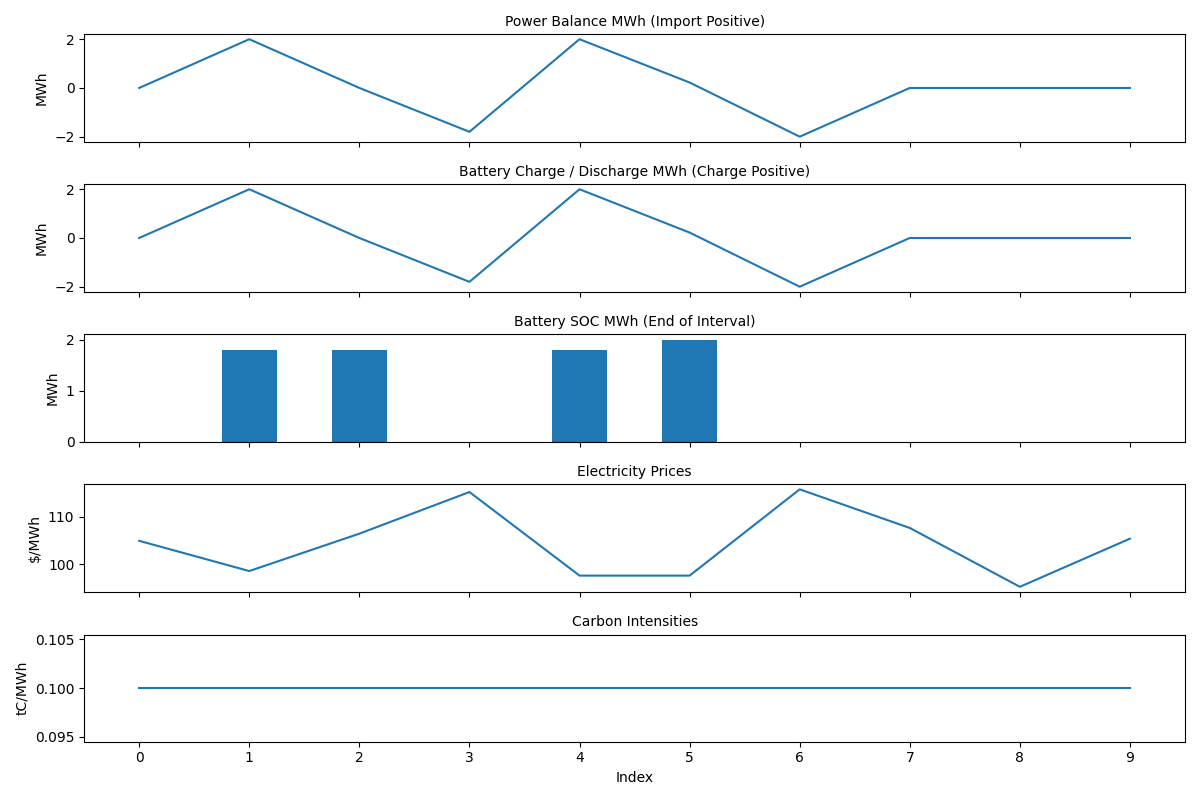
We can demonstrate the state of charge and battery power settings by first optimizing a battery and showing it's plot:
import numpy as np
import energypylinear as epl

np.random.seed(42)
electricity_prices = np.random.normal(100, 10, 10).tolist()
asset = epl.battery.Battery(power_mw=2, capacity_mwh=4)
results = asset.optimize(electricity_prices=electricity_prices)
asset.plot(results, path="./docs/docs/static/battery.png")

Takeaways:
- the battery state of charge is constrained between 0 and 4 MWh,
- the battery power rating is constrained between -2 and 2 MW,
- battery SOC starts empty and ends empty.
import numpy as np
import energypylinear as epl

np.random.seed(42)
electricity_prices = np.random.normal(100, 10, 10).tolist()
asset = epl.battery.Battery(
    power_mw=4,
    capacity_mwh=8,
)
results = asset.optimize(
    electricity_prices=electricity_prices,
    initial_charge_mwh=1.0,
    final_charge_mwh=3.0
)
asset.plot(results, path="./docs/docs/static/battery-fast.png")

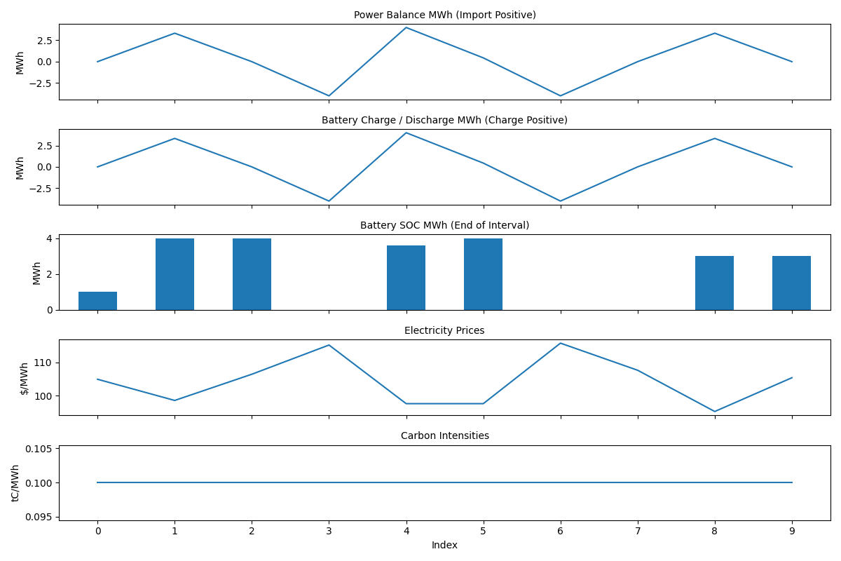
Takeaways:
- battery SOC starts at 1 MWh and ends at 3 MWh.